1、数学公式

数学公式的前后要加上  $  或   \  ，比如：$f(x) = 3x + 7$  和    \(f(x) = 3x + 7) \   效果是一样的；如果用   \ \，或者使用   $$ 和   $$，则该公式独占一行；如果用 \begin{equation}和 \end{equation}，则公式除了独占一行还会自动被添加序号， 如何公式不想编号则使用 \begin{equation*} 和 \end{equation*}.

2、字符

普通字符在数学公式中含义一样，除了# $ % & ~ _ ^ \ { }若要在数学环境中表示这些符号   # $ % & _ { }，需要分别表示为  # $ % & _ { }，即在个字符前加上 \ 。

3、上标和下标

用 ^ 来表示上标，用 _ 来表示下标，看一简单例子：

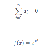
1 2	$$sum_{i=1}^n a_i=0$$ $$ f(x)=x^{x^x}$$

效果如下:

 

 

 

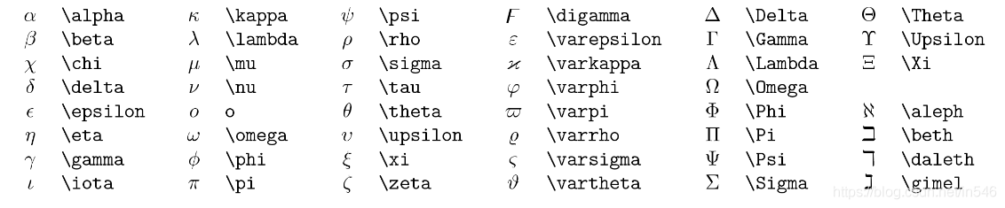
4、希腊字母

 

 

 

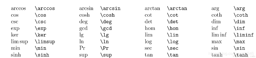
5、数学函数

 

 

 

6、在公式中插入文本

可以通过 \mbox{text} 在公式中添加  text ，比如：

1 2 3 4 5 6 7

\documentclass{article} \usepackage{CJK} \begin{CJK*}{GBK}{song} \begin{document} $$\mbox{对任意的$x>0$}, \mbox{有 }f(x)>0. $$ \end{CJK*} \end{document}

效果: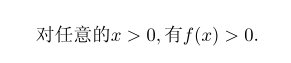

　

7、分数及开方

1 2 3

\frac{分子}{分母}       \sqrt{expression_r_r_r}表示开平方， \sqrt[n]{expression_r_r_r} 表示开 n 次方.

8、省略号（3个点）

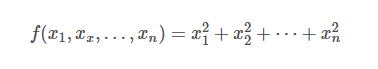
\ldots 表示跟文本底线对齐的省略号；\cdots 表示跟文本中线对齐的省略号，比如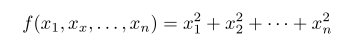：表示为

 

 

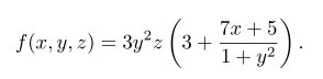
9、括号和分隔符

() 和 [ ] 和 ｜ 对应于自己；{} 对应于 { }；|| 对应于 |。当要显示大号的括号或分隔符时，要对应用 \left 和 \right，如：[f(x,y,z) = 3y^2 z \left( 3 + \frac{7x+5}{1 + y^2} \right).]对应于

\left. 和 \right. 只用与匹配，本身是不显示的，比如，要输出：

 

 

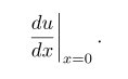
则用left. \frac{du}{dx} \right|_{x=0}.

10、多行的数学公式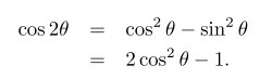

 

 可以表示为：

1 2 3 4

\begin{eqnarray*} \cos 2\theta & = & \cos^2 \theta - \sin^2 \theta \\ & = & 2 \cos^2 \theta - 1. \end{eqnarray*}

其中&是对其点，表示在此对齐。*  使latex不自动显示序号，如果想让latex自动标上序号，则把   *   去掉

 

11、矩阵

 

 

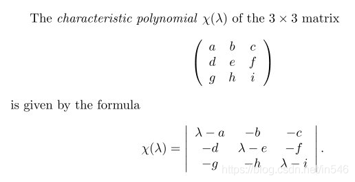
表示为：

1 2 3 4 5 6 7 8 9 10 11

The \emph{characteristic polynomial} $\chi(\lambda)$ of the $3 \times 3$~matrix \[ \left( \begin{array}{ccc} a & b & c \\ d & e & f \\ g & h & i \end{array} \right)\] is given by the formula \[ \chi(\lambda) = \left| \begin{array}{ccc} \lambda - a & -b & -c \\ -d & \lambda - e & -f \\ -g & -h & \lambda - i \end{array} \right|.\]

12、导数、极限、求和、积分(Derivatives, Limits, Sums and Integrals)

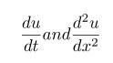
\frac{du}{dt} and \frac{d^2 u}{dx^2}

 

效果如下：

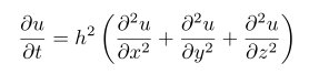
1 2 3 4

\[ \frac{\partial u}{\partial t} = h^2 \left( \frac{\partial^2 u}{\partial x^2} + \frac{\partial^2 u}{\partial y^2} + \frac{\partial^2 u}{\partial z^2}\right)\]

效果如下：

 

 

 

1	\lim_{x \to +\infty}, \inf_{x > s} and \sup_K

效果如下：

 

 

 

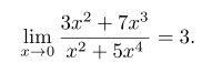
1	\[ \lim_{x \to 0} \frac{3x^2 +7x^3}{x^2 +5x^4} = 3.\]

效果如下：

 

 

 

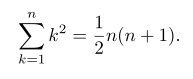
1	> \[ \sum_{k=1}^n k^2 = \frac{1}{2} n (n+1).\]

效果如下：

 

 

 

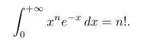
1	\[ \int_0^{+\infty} x^n e^{-x} \,dx = n!.\]

效果如下：

 

 

 

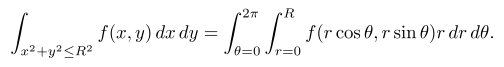
1 2 3

\[ \int_{x^2 + y^2 \leq R^2} f(x,y)\,dx\,dy = \int_{\theta=0}^{2\pi} \int_{r=0}^R f(r\cos\theta,r\sin\theta) r\,dr\,d\theta.\]

效果如下：

 

 

 

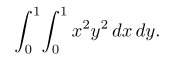
1	\[ \int_0^1 \! \int_0^1 x^2 y^2\,dx\,dy.\]

效果如下：

 

 

 

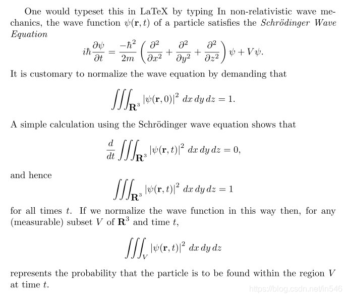
1 2 3 4 5 6 7 8 9 10 11 12 13 14 15 16 17 18 19 20 21 22 23 24 25 26 27

One would typeset this in LaTeX by typing In non-relativistic wave mechanics, the wave function $\psi(\mathbf{r},t)$ of a particle satisfies the \emph{Schr\"{o}dinger Wave Equation} \[ i\hbar\frac{\partial \psi}{\partial t} = \frac{-\hbar^2}{2m} \left( \frac{\partial^2}{\partial x^2} + \frac{\partial^2}{\partial y^2} + \frac{\partial^2}{\partial z^2} \right) \psi + V \psi.\] It is customary to normalize the wave equation by demanding that \[ \int \!\!\! \int \!\!\! \int_{\textbf{R}^3} \left| \psi(\mathbf{r},0) \right|^2\,dx\,dy\,dz = 1.\] A simple calculation using the Schr\"{o}dinger wave equation shows that \[ \frac{d}{dt} \int \!\!\! \int \!\!\! \int_{\textbf{R}^3} \left| \psi(\mathbf{r},t) \right|^2\,dx\,dy\,dz = 0,\] and hence \[ \int \!\!\! \int \!\!\! \int_{\textbf{R}^3} \left| \psi(\mathbf{r},t) \right|^2\,dx\,dy\,dz = 1\] for all times~$t$. If we normalize the wave function in this way then, for any (measurable) subset~$V$ of $\textbf{R}^3$ and time~$t$, \[ \int \!\!\! \int \!\!\! \int_V \left| \psi(\mathbf{r},t) \right|^2\,dx\,dy\,dz\] represents the probability that the particle is to be found within the region~$V$ at time~$t$.

效果如下：

转载本文请联系原作者获取授权，同时请注明本文来自宋红强科学网博客。
链接地址：https://wap.sciencenet.cn/blog-597968-1480764.html