博文
python做因素方差分析
||
在实验优化与设计中,书中的例子比较陈旧,使用minitab或SPSS软件处理起来不够直观。尝试使用python来实现。
例子1:为了招聘机械技工,由人事部门和生产车间共同考查。加工车间已有三台同型号和同规格的机床,设备之间无明显差异。分别由预选的三个工人操作,在相同的条件下加工同一零件。需考查三个工人的生产率有无差异,现将同时观测五天的日产量(件数)填入数据采集表中。已知日产量服从正态分布。
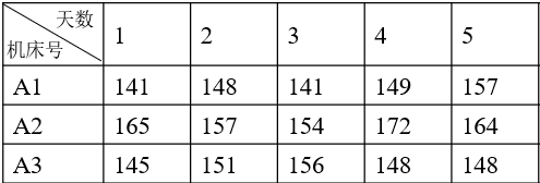
单因素三水平五次重复实验。
import numpy as np
import pandas as pd
import scipy.stats as stats
import matplotlib.pyplot as plt
import seaborn as sns
from statsmodels.formula.api import ols
from statsmodels.stats.anova import anova_lm
from scipy.stats import ttest_1samp
将数据重新写成一个worker.csv文件
df4 = pd.read_csv('worker.csv',sep = ',', encoding = 'gbk')
df4.head(3)
df4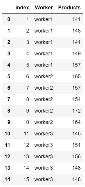
画图直观看
df4.boxplot('Products', by='Worker', figsize=(12, 8))
#sns.boxplot(x='Products',y='Worker',data=df4)
plt.savefig('Products-Worker')
可以直观看到worker2产量最高。
进行显著性检验
from scipy import stats
F, p = stats.f_oneway(d_data['worker1'], d_data['worker2'], d_data['worker3'])
print(F, p)
输出
8.958855098389986 0.004164063755613985
即计算的F值为8.96,置信度(1-0.004)>99%。查F分布表,F0.01(2,12)=6.93。8.96>6.93, 产量存在显著差异。直接使用ols来处理,生成anova_table。
model=ols('Products ~Worker', data=df4).fit()
anova_table = anova_lm(model, type=2)
pd.DataFrame(anova_table)
-----------------------------------------------------------------------------------------------------------
例子2:考察温度对一化工产品的得率的影响,选了五种不同的温度,同一温度做了三次实验,结果如下:
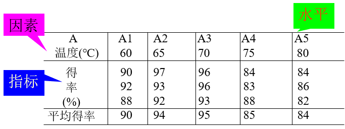
单因素五水平三次重复实验。为方便处理,改写表格为因素一列。
df_temperature = pd.read_csv('temperature.csv',sep = ',', encoding = 'gbk')
df_temperature
print(df_temperature)
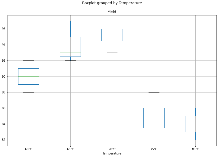
df_temperature.boxplot('Yield', by='Temperature', figsize=(12, 8))
plt.savefig('Temperature-Yield')
Index Temperature Yield
0 1 60℃ 90
1 2 60℃ 92
2 3 60℃ 88
3 4 65℃ 97
4 5 65℃ 93
5 6 65℃ 92
6 7 70℃ 96
7 8 70℃ 96
8 9 70℃ 93
9 10 75℃ 84
10 11 75℃ 83
11 12 75℃ 88
12 13 80℃ 84
13 14 80℃ 86
14 15 80℃ 82箱线图为
显著性检验
yield_60 = df_temperature['Yield'][df_temperature.Temperature == '60℃']

temperatures = pd.unique(df_temperature.Temperature.values)
#dictionary d_data, grp is the key and the corresponding weights are the value, defined by a for loop
d_data_tem = {temperature:df_temperature['Yield'][df_temperature.Temperature == temperature] for temperature in temperatures}
#print(d_data_tem)

k = len(pd.unique(df_temperature.Temperature))  # number of conditions
N = len(df_temperature.values)  # conditions times participants
#n = df_temperature.groupby('Temperature').size()[0] #Participants in each condition
#print(df_temperature.groupby('Temperature').size())

from scipy import stats

F, p = stats.f_oneway(d_data_tem['60℃'], d_data_tem['65℃'], d_data_tem['70℃'],d_data_tem['75℃'], d_data_tem['80℃'])

print(F, p)
输出检验结果
15.180000000000001 0.0002992192431928024
使用anova_table
model=ols('Yield ~Temperature', data=df_temperature).fit()
anova_table = anova_lm(model, type=2)
pd.DataFrame(anova_table)
以上是单因素实验。对于双因素实验,从网上看的一个例子数据,并非真实采集,仅用来摸索一下分析方法。
例子3:探索收入与教育程度、职业的关系。
df = pd.read_csv('income.csv',sep = ',', encoding = 'gbk')
df['ln_income'] = np.log(df['income'])
df.head(15)
输入结果如下:

fig, ax = plt.subplots(1,2,figsize=(12,6))
ax1 = sns.boxplot(x='education',y='ln_income',data=df, ax=ax[0])
ax1.set_title('education-ln_income')
ax2=sns.boxplot(x='career',y='ln_income',data=df, ax=ax[1])
ax2.set_title('career-ln_income')
plt.show()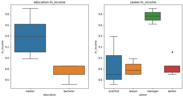
进行双因素ANOVA分析
model=ols('ln_income ~career + education + career: education', data=df).fit()
anova_table = anova_lm(model, type=2)
pd.DataFrame(anova_table)
例子4:对某型号铣刀进行等温淬火工艺实验,以考查等温温度(因素A)和淬火温度(因素B)对铣刀硬度的影响。已知等温温度和淬火温度对铣刀硬度的影响无交互作用。根据专业知识和实践经验,等温温度和淬火温度各取三个水平,因素水平及实验结果如表所列。判断在所选水平范围内,等温温度和淬火温度对铣刀硬度的影响是否显著?.

双因素三水平实验。
df_knife = pd.read_csv('knife.csv',sep = ',', encoding = 'gbk')
df_knife
fig, ax = plt.subplots(1,2,figsize=(12,6))
ax1 = sns.boxplot(x='isothermal',y='hardness',data=df_knife, ax=ax[0])
ax1.set_title('isothermal-hardness')
ax2=sns.boxplot(x='quenching',y='hardness',data=df_knife, ax=ax[1])
ax2.set_title('quenching-hardness')
plt.savefig('heattreatment-hardness')
plt.show()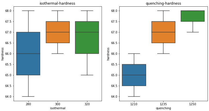
model_knife=ols('hardness ~isothermal + quenching + isothermal: quenching', data=df_knife).fit()
anova_table = anova_lm(model_knife, type=2)
pd.DataFrame(anova_table)
等温温度是非显著性因素,淬火温度是显著因素。
https://wap.sciencenet.cn/blog-907836-1337256.html
上一篇:《蛤蟆先生去看心理医生》摘录
下一篇:python做三因素方差分析