博文

[转载]Color spaces in OpenCV

已有 2920 次阅读 2019-2-6 03:46 |系统分类:科研笔记|文章来源:转载

In this tutorial, we will learn about popular colorspaces used in Computer Vision and use it for color based segmentation. We will also share demo code in C++ and Python.

In 1975, the Hungarian Patent HU170062 introduced a puzzle with just one right solution out of 43,252,003,274,489,856,000 (43 quintillion) possibilities. This invention now known as the Rubik’s Cube took the world by storm selling more than 350 million by January 2009.

So, when a few days back my friend, Mark, told me about his idea of building a computer vision based automated Rubik’s cube solver, I was intrigued. He was trying to use color segmentation to find the current state of the cube. While his color segmentation code worked pretty well during evenings in his room, it fell apart during daytime outside his room!

He asked me for help and I immediately understood where he was going wrong. Like many other amateur computer vision enthusiasts, he was not taking into account the effect of different lighting conditions while doing color segmentation. We face this problem in many computer vision applications involving color based segmentation like skin tone detection, traffic light recognition etc. Let’s see how we can help him build a robust color detection system for his robot.

The article is organized as follows:

First we will see how to read an image in OpenCV and convert it into different color spaces and see what new information do the different channels of each color space provide us.
We will apply a simple color segmentation algorithm as done by Mark and ponder over its weaknesses.
Then we will jump into some analytics and use a systematic way to choose:

The right color space.
The right threshold values for segmentation.

See the results

The different color spaces

In this section, we will cover some important color spaces used in computer vision. We will not describe the theory behind them as it can be found on Wikipedia. Instead, we will develop a basic intuition and learn some important properties which will be useful in making decisions later on.

Let us load 2 images of the same cube. It will get loaded in BGR format by default. We can convert between different colorspaces using the OpenCV function cvtColor() as will be shown later.

#python

bright = cv2.imread('cube1.jpg')

dark = cv2.imread('cube8.jpg')

//C++

bright = cv::imread('cube1.jpg')

dark = cv::imread('cube8.jpg')

The first image is taken under outdoor conditions with bright sunlight, while the second is taken indoor with normal lighting conditions.

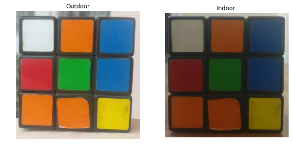Figure 1 : Two images of the same cube taken under different illumination

The RGB Color Space

The RGB colorspace has the following properties

It is an additive colorspace where colors are obtained by a linear combination of Red, Green, and Blue values.
The three channels are correlated by the amount of light hitting the surface.

Let us split the two images into their R, G and B components and observe them to gain more insight into the color space.

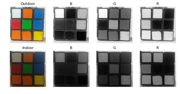Figure 2 : Different Channels Blue ( B ), Green ( G ), Red ( R ) of the RGB color space shown separately

Observations

If you look at the blue channel, it can be seen that the blue and white pieces look similar in the second image under indoor lighting conditions but there is a clear difference in the first image. This kind of non-uniformity makes color based segmentation very difficult in this color space. Further, there is an overall difference between the values of the two images. Below we have summarized the inherent problems associated with the RGB Color space:

significant perceptual non-uniformity.
mixing of chrominance ( Color related information ) and luminance ( Intensity related information ) data.

The LAB Color-Space

The Lab color space has three components.

L – Lightness ( Intensity ).
a – color component ranging from Green to Magenta.
b – color component ranging from Blue to Yellow.

The Lab color space is quite different from the RGB color space. In RGB color space the color information is separated into three channels but the same three channels also encode brightness information. On the other hand, in Lab color space, the L channel is independent of color information and encodes brightness only. The other two channels encode color.

It has the following properties.

Perceptually uniform color space which approximates how we perceive color.
Independent of device ( capturing or displaying ).
Used extensively in Adobe Photoshop.
Is related to the RGB color space by a complex transformation equation.

Let us see the two images in the Lab color space separated into three channels.

#python

brightLAB = cv2.cvtColor(bright, cv2.COLOR_BGR2LAB)

darkLAB = cv2.cvtColor(dark, cv2.COLOR_BGR2LAB)

//C++

cv::cvtColor(bright, brightLAB, cv::COLOR_BGR2LAB);

cv::cvtColor(dark, darkLAB, cv::COLOR_BGR2LAB);

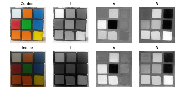Figure 3 : The Lightness ( L ), and color components ( A, B ) in LAB Color space.

Observations

It is pretty clear from the figure that the change in illumination has mostly affected the L component.
The A and B components which contain the color information did not undergo massive changes.
The respective values of Green, Orange and Red ( which are the extremes of the A Component ) has not changed in the B Component and similarly the respective values of Blue and Yellow ( which are the extremes of the B Component ) has not changed in the A component.

The YCrCb Color-Space

The YCrCb color space is derived from the RGB color space and has the following three compoenents.

Y – Luminance or Luma component obtained from RGB after gamma correction.
Cr = R – Y ( how far is the red component from Luma ).
Cb = B – Y ( how far is the blue component from Luma ).

This color space has the following properties.

Separates the luminance and chrominance components into different channels.
Mostly used in compression ( of Cr and Cb components ) for TV Transmission.
Device dependent.

The two images in YCrCb color space separated into its channels are shown below

#python

brightYCB = cv2.cvtColor(bright, cv2.COLOR_BGR2YCrCb)

darkYCB = cv2.cvtColor(dark, cv2.COLOR_BGR2YCrCb)

//C++

cv::cvtColor(bright, brightYCB, cv::COLOR_BGR2YCrCb);

cv::cvtColor(dark, darkYCB, cv::COLOR_BGR2YCrCb);

Figure 4 : Luma ( Y ), and Chroma ( Cr, Cb ) components in YCrCb color space.

Observations

Similar observations as LAB can be made for Intensity and color components with regard to Illumination changes.
Perceptual difference between Red and Orange is less even in the outdoor image as compared to LAB.
White has undergone change in all 3 components.

The HSV Color Space

The HSV color space has the following three components

H – Hue ( Dominant Wavelength ).
S – Saturation ( Purity / shades of the color ).
V – Value ( Intensity ).

Let’s enumerate some of its properties.

Best thing is that it uses only one channel to describe color (H), making it very intuitive to specify color.
Device dependent.

The H, S and V components of the two images are shown below.

#python

brightHSV = cv2.cvtColor(bright, cv2.COLOR_BGR2HSV)

darkHSV = cv2.cvtColor(dark, cv2.COLOR_BGR2HSV)

//C++

cv::cvtColor(bright, brightHSV, cv::COLOR_BGR2HSV);

cv::cvtColor(dark, darkHSV, cv::COLOR_BGR2HSV);

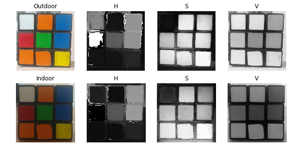Figure 5 : Hue ( H ), Saturation ( S ) and Value ( V ) components in HSV color space.

Observations

The H Component is very similar in both the images which indicates the color information is intact even under illumination changes.
The S component is also very similar in both images.
The V Component captures the amount of light falling on it thus it changes due to illumination changes.
There is drastic difference between the values of the red piece of outdoor and Indoor image. This is because Hue is represented as a circle and red is at the starting angle. So, it may take values between [300, 360] and again [0, 60].

How to use these color spaces for segmentation

The simplest way

Now that we have got some idea about the different color spaces, lets first try to use them to detect the Green color from the cube.

Step 1 : Get the color values for a particular color

Find the approximate range of values of green color for each color space. For doing this, I’ve made an interactive GUI where you can check the values of all the color spaces for each pixel just by hovering the mouse on the image as shown below :

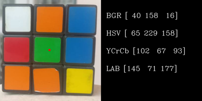Figure 6 : Demo showing a pixel and its value in different color spaces for the Outdoor image.

Step 2 : Applying threshold for segmentation

Extract all pixels from the image which have values close to that of the green pixel. We can take a range of +/- 40 for each color space and check how the results look like. We will use the opencv function inRange for finding the mask of green pixels and then use bitwise_and operation to get the green pixels from the image using the mask.

Also note that for converting one pixel to another color space, we first need to convert 1D array to a 3D array.

#python

bgr = [40, 158, 16]

thresh = 40

minBGR = np.array([bgr[0] - thresh, bgr[1] - thresh, bgr[2] - thresh])

maxBGR = np.array([bgr[0] + thresh, bgr[1] + thresh, bgr[2] + thresh])

maskBGR = cv2.inRange(bright,minBGR,maxBGR)

resultBGR = cv2.bitwise_and(bright, bright, mask = maskBGR)

#convert 1D array to 3D, then convert it to HSV and take the first element

# this will be same as shown in the above figure [65, 229, 158]

hsv = cv2.cvtColor( np.uint8([[bgr]] ), cv2.COLOR_BGR2HSV)[0][0]

minHSV = np.array([hsv[0] - thresh, hsv[1] - thresh, hsv[2] - thresh])

maxHSV = np.array([hsv[0] + thresh, hsv[1] + thresh, hsv[2] + thresh])

maskHSV = cv2.inRange(brightHSV, minHSV, maxHSV)

resultHSV = cv2.bitwise_and(brightHSV, brightHSV, mask = maskHSV)

#convert 1D array to 3D, then convert it to YCrCb and take the first element

ycb = cv2.cvtColor( np.uint8([[bgr]] ), cv2.COLOR_BGR2YCrCb)[0][0]

minYCB = np.array([ycb[0] - thresh, ycb[1] - thresh, ycb[2] - thresh])

maxYCB = np.array([ycb[0] + thresh, ycb[1] + thresh, ycb[2] + thresh])

maskYCB = cv2.inRange(brightYCB, minYCB, maxYCB)

resultYCB = cv2.bitwise_and(brightYCB, brightYCB, mask = maskYCB)

#convert 1D array to 3D, then convert it to LAB and take the first element

lab = cv2.cvtColor( np.uint8([[bgr]] ), cv2.COLOR_BGR2LAB)[0][0]

minLAB = np.array([lab[0] - thresh, lab[1] - thresh, lab[2] - thresh])

maxLAB = np.array([lab[0] + thresh, lab[1] + thresh, lab[2] + thresh])

maskLAB = cv2.inRange(brightLAB, minLAB, maxLAB)

resultLAB = cv2.bitwise_and(brightLAB, brightLAB, mask = maskLAB)

cv2.imshow("Result BGR", resultBGR)

cv2.imshow("Result HSV", resultHSV)

cv2.imshow("Result YCB", resultYCB)

cv2.imshow("Output LAB", resultLAB)

//C++ code

cv::Vec3b bgrPixel(40, 158, 16);

// Create Mat object from vector since cvtColor accepts a Mat object

Mat3b bgr (bgrPixel);

//Convert pixel values to other color spaces.

Mat3b hsv,ycb,lab;

cvtColor(bgr, ycb, COLOR_BGR2YCrCb);

cvtColor(bgr, hsv, COLOR_BGR2HSV);

cvtColor(bgr, lab, COLOR_BGR2Lab);

//Get back the vector from Mat

Vec3b hsvPixel(hsv.at<Vec3b>(0,0));

Vec3b ycbPixel(ycb.at<Vec3b>(0,0));

Vec3b labPixel(lab.at<Vec3b>(0,0));

int thresh = 40;

cv::Scalar minBGR = cv::Scalar(bgrPixel.val[0] - thresh, bgrPixel.val[1] - thresh, bgrPixel.val[2] - thresh)

cv::Scalar maxBGR = cv::Scalar(bgrPixel.val[0] + thresh, bgrPixel.val[1] + thresh, bgrPixel.val[2] + thresh)

cv::Mat maskBGR, resultBGR;

cv::inRange(bright, minBGR, maxBGR, maskBGR);

cv::bitwise_and(bright, bright, resultBGR, maskBGR);

cv::Scalar minHSV = cv::Scalar(hsvPixel.val[0] - thresh, hsvPixel.val[1] - thresh, hsvPixel.val[2] - thresh)

cv::Scalar maxHSV = cv::Scalar(hsvPixel.val[0] + thresh, hsvPixel.val[1] + thresh, hsvPixel.val[2] + thresh)

cv::Mat maskHSV, resultHSV;

cv::inRange(brightHSV, minHSV, maxHSV, maskHSV);

cv::bitwise_and(brightHSV, brightHSV, resultHSV, maskHSV);

cv::Scalar minYCB = cv::Scalar(ycbPixel.val[0] - thresh, ycbPixel.val[1] - thresh, ycbPixel.val[2] - thresh)

cv::Scalar maxYCB = cv::Scalar(ycbPixel.val[0] + thresh, ycbPixel.val[1] + thresh, ycbPixel.val[2] + thresh)

cv::Mat maskYCB, resultYCB;

cv::inRange(brightYCB, minYCB, maxYCB, maskYCB);

cv::bitwise_and(brightYCB, brightYCB, resultYCB, maskYCB);

cv::Scalar minLAB = cv::Scalar(labPixel.val[0] - thresh, labPixel.val[1] - thresh, labPixel.val[2] - thresh)

cv::Scalar maxLAB = cv::Scalar(labPixel.val[0] + thresh, labPixel.val[1] + thresh, labPixel.val[2] + thresh)

cv::Mat maskLAB, resultLAB;

cv::inRange(brightLAB, minLAB, maxLAB, maskLAB);

cv::bitwise_and(brightLAB, brightLAB, resultLAB, maskLAB);

cv2::imshow("Result BGR", resultBGR)

cv2::imshow("Result HSV", resultHSV)

cv2::imshow("Result YCB", resultYCB)

cv2::imshow("Output LAB", resultLAB)

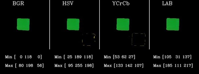Figure 7 : RGB looks good, May be we are just wasting time here.

Some more results

So, it seems that the RGB and LAB are enough to detect the color and we dont need to think much. Lets see some more results.

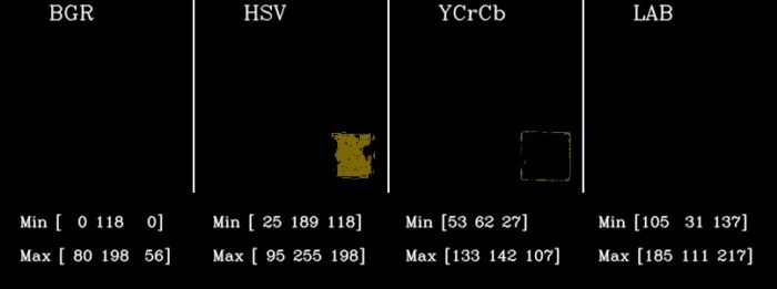Figure 8 : Applying the same threshold to the Indoor image fails to detect the green cubes in all the color spaces.

So, the same threshold doesn’t work on the dark image. Doing the same experiment to detect the yellow color gives the following results.

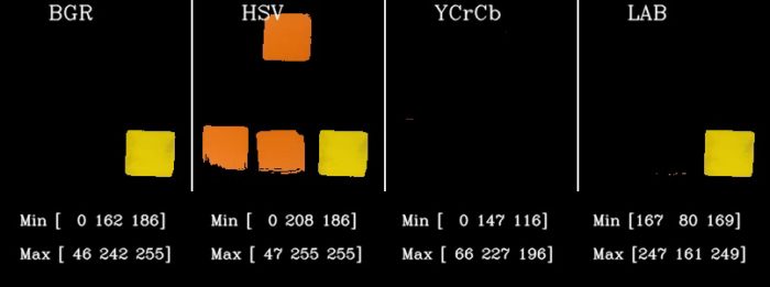Figure 9 : Trying to detect the yellow pieces using the same technique and threshold ( for yellow ) obtained from bright image. HSV and YCrCb are still not performing well.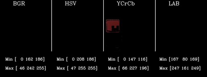Figure 10 : Trying to detect the yellow pieces using the threshold obtained from bright cube. All color spaces fail again.

But why is it that the results are so bad? This is because we had taken a wild guess of 40 for the threshold. I made another interactive demo where you can play with the values and try to find one that works for all the images. Check out the screenshot. But then there will be cases where another image comes and it doesn’t work again. We cannot just take some threshold by trial and error blindly. We are not using the power of the color spaces by doing so.

We need to have some methodical way to find the correct threshold values.

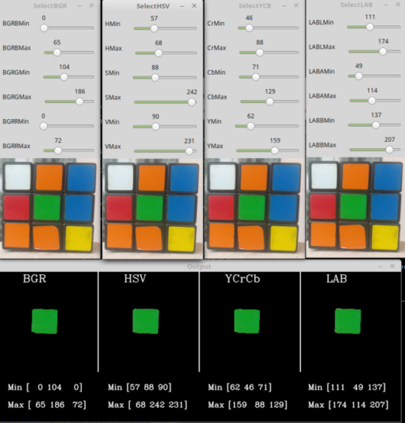Figure 11 : Screenshot of the demo for playing around with the different values to detect the particular color in all color spaces for a given image.

Some Data Analysis for a Better Solution

Step 1 : Data Collection

I have collected 10 images of the cube under varying illumination conditions and separately cropped every color to get 6 datasets for the 6 different colors. You can see how much change the colors undergo visually.

Figure : Showing changes in color due to varying Illumination conditions

Step 2 : Compute the Density plot

Check the distribution of a particular color say, blue or yellow in different color spaces. The density plot or the 2D Histogram gives an idea about the variations in values for a given color. For example, Ideally the blue channel of a blue colored image should always have the value of 255. But practically, it is distributed between 0 to 255.

I am showing the code only for BGR color space. You need to do it for all the color spaces.

We will first load all images of blue or yellow pieces.

#python

B = np.array([])

G = np.array([])

R = np.array([])

im = cv2.imread(fi)

Separate the channels and create and array for each channel by appending the values from each image.

#python

b = im[:,:,0]

b = b.reshape(b.shape[0]*b.shape[1])

g = im[:,:,1]

g = g.reshape(g.shape[0]*g.shape[1])

r = im[:,:,2]

r = r.reshape(r.shape[0]*r.shape[1])

B = np.append(B,b)

G = np.append(G,g)

R = np.append(R,r)

Use histogram plot from matplotlib to plot the 2D histogram

#python

nbins = 10

plt.hist2d(B, G, bins=nbins, norm=LogNorm())

plt.xlabel('B')

plt.ylabel('G')

plt.xlim([0,255])

plt.ylim([0,255])

Observations : Similar Illumination

Figure 13 : Density Plot showing the variation of values in color channels for 2 similar bright images of blue color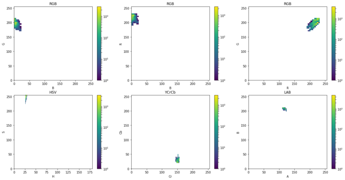Figure 14 : Density Plot showing the variation of values in color channels for 2 similar bright images for the yellow color

It can be seen that under similar lighting conditions all the plots are very compact. Some points to be noted are :

YCrCb and LAB are much more compact than others
In HSV, there is variation in S direction ( color purity ) but very little variation in H direction.

Observations : Different Illumination

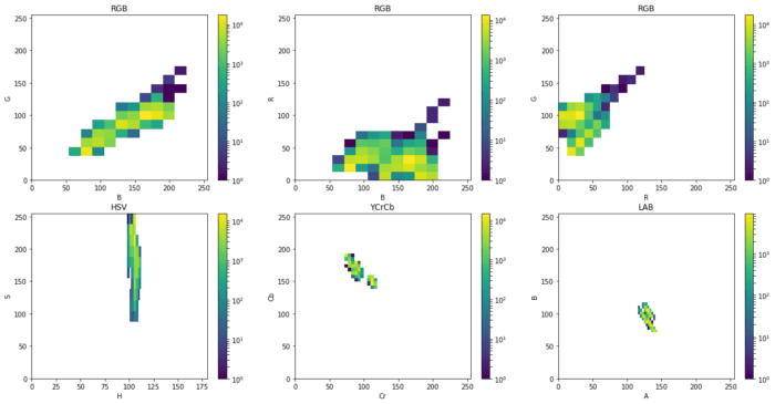Figure 15 : Density Plot showing the variation of values in color channels under varying illumination for the blue colorFigure 16 : Density Plot showing the variation of values in color channels under varying illumination for the yellow color

As the Illumination changes by a large amount, we can see that :

Ideally, we want to work with a color space with the most compact / concentrated density plot for color channels.
The density plots for RGB blow up drastically. This means that the variation in the values of the channels is very high and fixing a threshold is a big problem. Fixing a higher range will detect colors which are similar to the desired color ( False Positives ) and lower range will not detect the desired color in different lighting ( False Negatives ).
In HSV, since only the H component contains information about the absolute color. Thus, it becomes my first choice of color space since I can tweak just one knob ( H ) to specify a color as compared to 2 knobs in YCrCb ( Cr and Cb ) and LAB ( A and B ).
Comparing the plots of YCrCb and LAB shows a higher level of compactness in case of LAB. So, next best choice for me becomes the LAB color space.

Final Results

In this last section, I will show the results for detecting the blue and yellow piece by taking the threshold values from the density plots and applying it to the respective color spaces in the same way we did in the second section. We don’t have to worry about the Intensity component when we are working in HSV, YCrCb and LAB color space. We just need to specify the thresholds for the color components. The values I’ve taken for generating the results are shown in the figures.

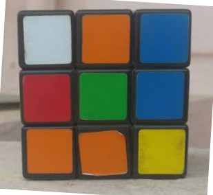Figure 17 : Demo Image 1Figure 18 : Results for Yellow color detection on Demo Image 1Figure 19 : Results for Blue color detection on Demo Image 1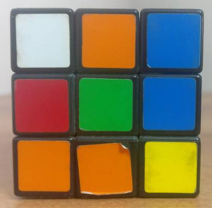Figure 20 : Demo Image 2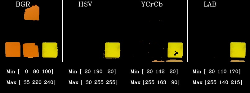Figure 21 : Results for Yellow color detection on Demo Image 2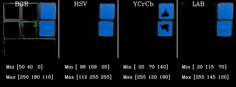Figure 22 : Results for Blue color detection on Demo Image 2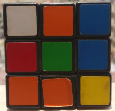Figure 23 : Demo Image 3Figure 24 : Results for Yellow color detection on Demo Image 3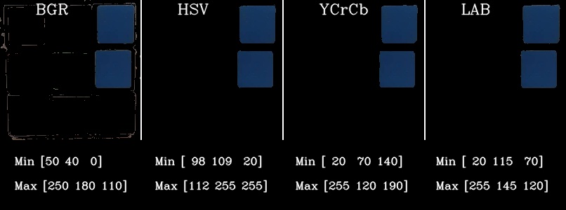Figure 25 : Results for Blue color detection on Demo Image 3

In the above results I have taken the values directly from the density plot. We can also chose to take the values which belong to to most dense region in the density plot which will help in getting tighter control of the color range. That will leave some holes and stray pixels which can be cleaned using Erosion and Dilation followed by Filtering.

Other Useful Applications of Color spaces

Histogram equalization is generally done on grayscale images. However, you can perform equalization of color images by converting the RGB image to YCbCr and doing histogram equalization of only the Y channel.
Color Transfer between two images by converting the images to Lab color space.
Many filters in smartphone camera applications like Google camera or Instagram make use of these Color space transforms to create those cool effects!

Sources:

https://www.learnopencv.com/color-spaces-in-opencv-cpp-python/

https://solarianprogrammer.com/2015/05/08/detect-red-circles-image-using-opencv/

转载本文请联系原作者获取授权，同时请注明本文来自陆宇振科学网博客。
链接地址：https://wap.sciencenet.cn/blog-578676-1160885.html

上一篇：[转载]Why is “using namespace std” considered bad practice
下一篇：What and where are the stack and heap

收藏 IP: 35.10.57.*| 热度|

当前推荐数：0

该博文允许注册用户评论请点击登录评论 (0 个评论)

数据加载中...

返回顶部

陆宇振

扫一扫，分享此博文

jingweimo的个人博客分享 http://blog.sciencenet.cn/u/jingweimo

博文

[转载]Color spaces in OpenCV

The different color spaces

The RGB Color Space

Observations

The LAB Color-Space

Observations

The YCrCb Color-Space

Observations

The HSV Color Space

Observations

How to use these color spaces for segmentation

The simplest way

Step 1 : Get the color values for a particular color

Step 2 : Applying threshold for segmentation

Some more results

Some Data Analysis for a Better Solution

Step 1 : Data Collection

Step 2 : Compute the Density plot

Observations : Similar Illumination

Observations : Different Illumination

Final Results

Other Useful Applications of Color spaces

当前推荐数：0

该博文允许注册用户评论请点击登录评论 (0 个评论)

陆宇振

全部作者的其他最新博文

全部精选博文导读

相关博文

jingweimo的个人博客分享 http://blog.sciencenet.cn/u/jingweimo

博文

[转载]Color spaces in OpenCV

The different color spaces

The RGB Color Space

Observations

The LAB Color-Space

Observations

The YCrCb Color-Space

Observations

The HSV Color Space

Observations

How to use these color spaces for segmentation

The simplest way

Step 1 : Get the color values for a particular color

Step 2 : Applying threshold for segmentation

Some more results

Some Data Analysis for a Better Solution

Step 1 : Data Collection

Step 2 : Compute the Density plot

Observations : Similar Illumination

Observations : Different Illumination

Final Results

Other Useful Applications of Color spaces

当前推荐数：0

该博文允许注册用户评论 请点击登录 评论 (0 个评论)

陆宇振

全部作者的其他最新博文

全部精选博文导读

相关博文

该博文允许注册用户评论请点击登录评论 (0 个评论)