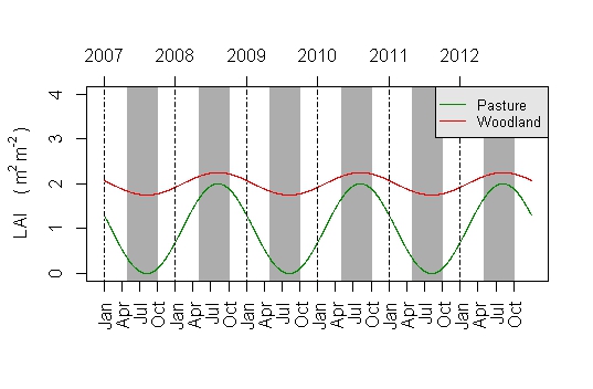
这幅图是2007年到2012年的LAI的多年变化,假设我们想对比两个站点的LAI, 这里用的是SIN 函数模拟的数据，你可以换成自己的数据，温度的或者其他的都可以。希望对您有帮助！

在R中，用以下代码，可以画出来。

# first construct the plot function

# timeP is to store time lables

fly_plot <- function(timeP, dataP1, dataP2, ylimup, ylabs,typeP='l')

{

 plot(timeP, dataP1, type=typeP,  xaxt = "n", col='green4',cex=0.5,

      ylim=c(0,ylimup), xlab="",ylab='')

 polygon(c(strptime('2007/5/1',"%Y/%m/%d"), strptime('2007/10/1',"%Y/%m/%d"),strptime('2007/10/1',"%Y/%m/%d"),strptime('2007/5/1',"%Y/%m/%d") ), c(-0.036*ylimup, -0.036*ylimup, ylimup+0.036*ylimup, ylimup+0.036*ylimup),col='grey68',border='grey68')

 polygon(c(strptime('2008/5/1',"%Y/%m/%d"), strptime('2008/10/1',"%Y/%m/%d"),strptime('2008/10/1',"%Y/%m/%d"),strptime('2008/5/1',"%Y/%m/%d") ), c(-0.036*ylimup, -0.036*ylimup, ylimup+0.036*ylimup, ylimup+0.036*ylimup),col='grey68',border='grey68')

 polygon(c(strptime('2009/5/1',"%Y/%m/%d"), strptime('2009/10/1',"%Y/%m/%d"),strptime('2009/10/1',"%Y/%m/%d"),strptime('2009/5/1',"%Y/%m/%d") ), c(-0.036*ylimup, -0.036*ylimup, ylimup+0.036*ylimup, ylimup+0.036*ylimup),col='grey68',border='grey68')

 polygon(c(strptime('2010/5/1',"%Y/%m/%d"), strptime('2010/10/1',"%Y/%m/%d"),strptime('2010/10/1',"%Y/%m/%d"),strptime('2010/5/1',"%Y/%m/%d") ), c(-0.036*ylimup, -0.036*ylimup, ylimup+0.036*ylimup, ylimup+0.036*ylimup),col='grey68',border='grey68')

 polygon(c(strptime('2011/5/1',"%Y/%m/%d"), strptime('2011/10/1',"%Y/%m/%d"),strptime('2011/10/1',"%Y/%m/%d"),strptime('2011/5/1',"%Y/%m/%d") ), c(-0.036*ylimup, -0.036*ylimup, ylimup+0.036*ylimup, ylimup+0.036*ylimup),col='grey68',border='grey68')

 polygon(c(strptime('2012/5/1',"%Y/%m/%d"), strptime('2012/10/1',"%Y/%m/%d"),strptime('2012/10/1',"%Y/%m/%d"),strptime('2012/5/1',"%Y/%m/%d") ), c(-0.036*ylimup, -0.036*ylimup, ylimup+0.036*ylimup, ylimup+0.036*ylimup),col='grey68',border='grey68')

 lines(timeP, dataP1, type=typeP,  xaxt = "n", col='green4',cex=0.5,

       ylim=c(0,ylimup), xlab="",ylab='')

 lines(timeP, dataP2, type=typeP, xaxt = "n", col='red2',cex=0.5,

       ylim=c(0,ylimup), xlab="",ylab='')

 axis.POSIXct(1, at = seq(r[1], r[2], by = "3 months"), format = "%b",las=2)

 #axis.POSIXct(1, at = seq(r[1], r[2], by = "2 months"), labels=NA)

 axis.POSIXct(3, at = seq(r[1], r[2], by = "1 years"), format="%Y")

 axis.POSIXct(1, at = seq(r[1], r[2], by = "1 years"), labels=NA, lty=4, tck=1)

 mtext(side=2, ylabs,line=2.5)

}

# plot LAI time series ----

# The LAI data is constructed by myself, and you can replace it with your data.

x = seq(0.9,6.9,by=1/365)

dataP1  = sin(pi*x)+1

dataP2  = 0.25*sin(pi*x)+2

timeP = seq(strptime('2007/1/1',"%Y/%m/%d"), by = "1 days", length.out = length(dataP1))

r <- as.POSIXct(round(range(timeP), "days"))

Sys.setlocale("LC_TIME", "US")

ylimup = 4

ylabs  = expression(paste('LAI    ( m'^'2 ','m'^'-2 ',')'))

fly_plot(timeP, dataP1, dataP2, ylimup, ylabs,typeP='l')

legend('topright', 1.04*ylimup, c("Pasture", "Woodland"),

      col = c('green4','red2'), cex=0.8, lty = c(1,1),merge = TRUE, bg = "gray90")

# 保存成tiff格式，分辨率设为300

tiff('LAI_fly.tiff',width=8,height=3.5,pointsize = 12,units='in',res=300)

LAI_fly = fly_plot(timeP, dataP1, dataP2, ylimup, ylabs,typeP='l')

legend("bottomright",c("Pasture", "Woodland"),

      col = c('green4','red2'), cex=0.8, lty = c(1,1),merge = TRUE, bg = "gray90")

dev.off()