博文
技术贴 | R语言——肠型分析:介绍、方法
|
导读
2011年,肠型(Enterotypes)的概念首次在《自然》杂志上由Arumugam等【1】提出,该研究发现可以将人类肠道微生物组分成稳定的3种类型,因为这3种类型不受年龄、性别、体重以及地域限制,表现出较高的稳定性,与血型具有很高的相似性,所以将其定义为肠型。后来的有的研究称发现2种肠型,也有称发现4种,这引起了国际上对于肠型概念的广泛讨论与争议。最新的《自然∙微生物学》杂志报道了学界对于肠型的最新认识,调解了之前关于肠型的一些争论【2】。
方法
目前流行的肠型计算方法有2种,一种是基于样品间的Jensen-Shannon距离,利用围绕中心点划分算法(PAM)进行聚类,最佳分类数目通过Calinski-Harabasz (CH)指数确定【3】;另一种则是直接基于物种丰度,利用狄利克雷多项混合模型(DMM)进行肠型分类【4】。
参考:人体肠道宏基因组生物信息分析方法 [J].微生物学报, 2018
Nature 2011 肠型分析教程:https://enterotype.embl.de/enterotypes.html#
Reference-Based肠型分析:http://enterotypes.org/
Github:https://github.com/tapj/biotyper
一、举例
文章一
来自:Quantitative microbiome profiling disentangles inflammation- and bile duct obstruction-associated microbiota alterations across PSC/IBD diagnoses.nature microbiology. 2019
方法:DirichletMultinomial.
描述:Enterotyping (or community typing) based on the DMM approach was performed in R as described previously. Enterotyping was performed on a combined genus-level abundance matrix including PSC/IBD and mHC samples compiled with 1,054 samples originating from the FGFP.
图1
文章二
来自:Impact of early events and lifestyle on the gut microbiota and metabolic phenotypes in young school-age children. micorbiome. 2019
方法:DMM, PAM-JSD, PAM-BC
描述:Genus-level enterotypes analysis was performed according to the Dirichlet multinomial mixtures (DMM) and partitioning around medoid (PAM)-based clustering protocols using Jensen-Shannon divergence (PAM-JSD) and Bray-Curtis (PAM-BC)
图2
二、函数:JSD计算距离、PAM聚类
library(ade4)
library(cluster)
library(clusterSim)

## 1. 菌属-样品相对丰度表
data=read.table("input.txt", header=T, row.names=1, dec=".", sep="\t")
data=data[-1,]

## 写函数
## JSD计算样品距离,PAM聚类样品,CH指数估计聚类数,比较Silhouette系数评估聚类质量。
dist.JSD <- function(inMatrix, pseudocount=0.000001, ...)
{
  ## 函数:JSD计算样品距离
  KLD <- function(x,y) sum(x *log(x/y))
  JSD<- function(x,y) sqrt(0.5 * KLD(x, (x+y)/2) + 0.5 * KLD(y, (x+y)/2))
  matrixColSize <- length(colnames(inMatrix))
  matrixRowSize <- length(rownames(inMatrix))
  colnames <- colnames(inMatrix)
  resultsMatrix <- matrix(0, matrixColSize, matrixColSize)

  inMatrix = apply(inMatrix,1:2,function(x) ifelse (x==0,pseudocount,x))

  for(i in 1:matrixColSize)
  {
    for(j in 1:matrixColSize)
    {
      resultsMatrix[i,j]=JSD(as.vector(inMatrix[,i]), as.vector(inMatrix[,j]))
    }
  }
  colnames -> colnames(resultsMatrix) -> rownames(resultsMatrix)
  as.dist(resultsMatrix)->resultsMatrix
  attr(resultsMatrix, "method") <- "dist"
  return(resultsMatrix)
}

pam.clustering = function(x, k)
{
  ## 函数:PAM聚类样品
  # x is a distance matrix and k the number of clusters
  require(cluster)
  cluster = as.vector(pam(as.dist(x), k, diss=TRUE)$clustering)
  return(cluster)
}
三、计算CH确定最佳Cluster
## 2. 选择CH指数最大的K值作为最佳聚类数
data.dist = dist.JSD(data)

# data.cluster=pam.clustering(data.dist, k=3) # k=3 为例
# nclusters = index.G1(t(data), data.cluster, d = data.dist, centrotypes = "medoids") # 查看CH指数
# nclusters = NULL

for(k in 1:20)
{
  if(k==1)
  {
    nclusters[k] = NA
  }
  else
  {
    data.cluster_temp = pam.clustering(data.dist, k)
    nclusters[k] = index.G1(t(data), data.cluster_temp,  d = data.dist, centrotypes = "medoids")
  }
}

plot(nclusters, type="h", xlab="k clusters", ylab="CH index", main="Optimal number of clusters") # 查看K与CH值得关系
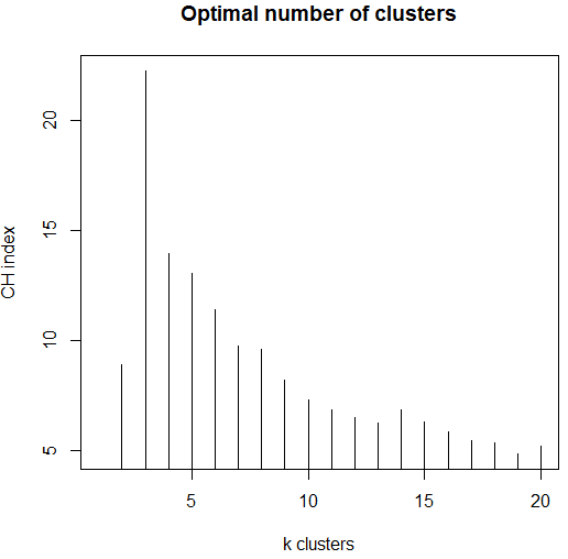
图3
如图,CH最大时的cluster数为3,最佳。
nclusters[1] = 0
k_best = which(nclusters == max(nclusters), arr.ind = TRUE)
三、JSD-PAM聚类,silhouette评估聚类质量
## 3. PAM根据JSD距离对样品聚类(分成K个组)
data.cluster=pam.clustering(data.dist, k = k_best)

## 4. silhouette评估聚类质量,-1=<S(i)=<1,越接近1越好
mean(silhouette(data.cluster, data.dist)[, k_best])
四、可视化:基于BCA
## plot 1
obs.pca=dudi.pca(data.frame(t(data)), scannf=F, nf=10)
obs.bet=bca(obs.pca, fac=as.factor(data.cluster), scannf=F, nf=k-1)

s.class(obs.bet$ls, fac=as.factor(data.cluster), grid=F,sub="Between-class analysis", col=c(1,2,3))
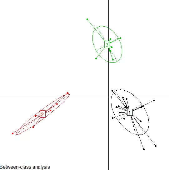
图4
五、可视化:基于PCoA
#plot 2
obs.pcoa=dudi.pco(data.dist, scannf=F, nf=3)

s.class(obs.pcoa$li, fac=as.factor(data.cluster), grid=F,sub="Principal coordiante analysis", col=c(1,2,3))
图5
参考:
【1】Enterotypes of the human gut microbiome. Nature, 2011
【2】人体肠道宏基因组生物信息分析方法 [J].微生物学报, 2018
【3】Linking long-term dietary patterns with gut microbial enterotypes. Science, 2011
【4】Dirichlet multinomial mixtures: generative models for microbial metagenomics. PLoS One, 2012
【5】Statin drugs might boost healthy gut microbes. Nature News. 2020
 你可能还喜欢
技术贴 | R语言:ggplot堆叠图、冲积图、分组分面、面积图
技术贴 | R语言:手把手教你画pheatmap热图
微生态科研学术群期待与您交流更多微生态科研问题
(联系微生态老师即可申请入群)
了解更多菌群知识,请关注“微生态”。
微信扫一扫
关注该公众号
https://wap.sciencenet.cn/blog-3474220-1285482.html
上一篇:医学微生物专栏 | 重要期刊最新研究进展
下一篇:农牧微生物专栏 | 重要期刊最值得看的研究成果盘点